DIY quantum random number generator, part2
- Part 1
- Part 2
So after nine long years the time has come for part two. Speaking of procrastination, huh.
This is a report on this project I’ve been working on as well as my cheat sheet for related utilities, so it won’t be brief or particularly clear, sorry.
I’ve been doing some research on this topic, and I found, to my surprise, that such devices can actually be called quantum RNGs! So I will be calling it exclusively ‘quantum’ from now on, mwahaha!
For years, I wanted to measure the output of this device and get some actual numbers from it. Therefore, the goal this time is to write some code for data gathering and analysis. It would be really nice to understand how much data the device in question might generate, find out data distributions, data patterns, and so on and so forth. Generated random sequences will be fed to ent and dieharder test suites for verification.
Setting up the camera
The first thing to mention is that the camera has some controls to tinker with, and changing these makes a big difference. You might get very low FPS due to long auto exposure times, or lots of false positives with low flash detection threshold and a noisy sensor. Checking available controls:
v4l2-ctl --list-ctrls
                     brightness 0x00980900 (int)    : min=0 max=255 step=1 default=128 value=128
                       contrast 0x00980901 (int)    : min=0 max=255 step=1 default=32 value=32
                     saturation 0x00980902 (int)    : min=0 max=255 step=1 default=32 value=32
 white_balance_temperature_auto 0x0098090c (bool)   : default=1 value=1
                           gain 0x00980913 (int)    : min=0 max=255 step=1 default=0 value=253
           power_line_frequency 0x00980918 (menu)   : min=0 max=2 default=2 value=2
      white_balance_temperature 0x0098091a (int)    : min=0 max=10000 step=10 default=4000 value=8880 flags=inactive
                      sharpness 0x0098091b (int)    : min=0 max=255 step=1 default=48 value=48
         backlight_compensation 0x0098091c (int)    : min=0 max=1 step=1 default=1 value=1
                  exposure_auto 0x009a0901 (menu)   : min=0 max=3 default=3 value=3
              exposure_absolute 0x009a0902 (int)    : min=1 max=10000 step=1 default=166 value=155 flags=inactive
         exposure_auto_priority 0x009a0903 (bool)   : default=0 value=1
I found the following to work quite well with my setup. I get around 30 FPS with bright and sharp flashes. For now, I’ll stick with running these manually right after plugging in the camera.
v4l2-ctl --set-ctrl=exposure_auto=1
v4l2-ctl --set-ctrl=exposure_absolute=295
v4l2-ctl --set-ctrl=exposure_auto_priority=0
v4l2-ctl --set-ctrl=sharpness=255
v4l2-ctl --set-ctrl=contrast=200
Live preview:
ffplay -f v4l2 -framerate 30 -video_size 640x480 -v verbose -i /dev/video0

Gathering data
OK, so it’s time to finally grab V4L2 library and write some code. My camera provides two output formats: YUYV and MJPG.
v4l2-ctl --device /dev/video0 --list-formats
ioctl: VIDIOC_ENUM_FMT
    Type: Video Capture

    [0]: 'YUYV' (YUYV 4:2:2)
    [1]: 'MJPG' (Motion-JPEG, compressed)
I found it easier to work with YUV 4:2:2 format because what we get is a 2D array with every other byte representing a pixel’s luminosity/brightness. Let X:Y be the detected flash if a pixel’s corresponding luminosity exceeds some threshold value, and we’re up and running.
Here are some assumptions I made at first, which eventually turned out to be wrong:
- Hits are be distributed uniformly across the sensor area.
- Each alpha particle gets detected by a single pixel.
- All matrix pixels behave the same way.
So, after modifying example code from the library, I have my first results:
Captured bufsize: 614400
Frame: 11,  bright pixels: 2
Frame: 12,  bright pixels: 2
Frame: 57,  bright pixels: 4
Frame: 121, bright pixels: 1
Frame: 135, bright pixels: 1
Frame: 176, bright pixels: 4
Frame: 177, bright pixels: 1
Frame: 198, bright pixels: 2
Frame: 208, bright pixels: 4
Frame: 209, bright pixels: 1
Frame: 250, bright pixels: 4
Frame: 252, bright pixels: 11
   ... 15 more lines ...
Frame: 452, bright pixels: 4
All of this means that some number of flashes gets registered every 16 frames, on average. All other frames are considered to be absolutely blank. OK, that’s the first measurement, so we’re getting there already!
Expected unexpectancies
After a short period of data gathering it became obvious, that often multiple neighboring pixels light up when a particle is detected. Which means something should be done to mitigate this effect. We cannot simply accept every coordinate because it’s highly likely the next one will be right next to it.
-
- 4th run, 3768 flashes gathered

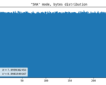
By this moment the main program can do two things: log coordinates of the flashes and convert each of X and Y coordinates to a corresponding byte value, thus producing two random bytes per flash. The method I used is pretty basic and it definitely gives terrible distribution, but that’s a start. Speaking of distributions, it’s necessary to plot data, so that’s what plot_data.py is for.
I left the device to collect data for about a week so I could get a substantial array of raw numbers to work with. Here’s a timelapse of one of the runs. Here, each pixel is colored in grayscale depending on how many times it was hit (three hits = white).

The same picture started showing up on the next few runs. Apparently, flashes are forming a somewhat bivariate normal distribution. Well of course, it’s basically a point source with omnidirectional particle emission, hence density is higher towards the center of the spot in the plane of the camera matrix! I feel so embarrassed for assuming uniformity at first LOL. Maybe it’s more correct to say that each axis forms a truncated normal distribution.
Now there are a bunch of problems to deal with. The sawtooth shape means there is a rounding error and bias towards 0 somewhere. The output is not uniform. The problem with multiple pixels per flash, as stated above is still unsolved.
For an unknown reason, edge pixels are about twice as sensitive compared with others. I decided the easiest way is to just ignore them, and implemented the --border option.
Yet another inconvenient problem arose: the amount of collected data grows with time, and my plot_data.py slows down drastically with each consequent run. Maybe it can be optimized, but it’s not worth it. It’s simpler to throw together another short tool to “replay” historical data: render_saved.sh. It’s rather rough but it does the job.
Prototyping data transformers
Minor problems aside, it’s time to focus on the major problem: uniformity. It turned out to be the most enjoyable and fun part of the whole story. Coding in C is not my strong suite and I’m not a masochist either, so I decided to make myself a safe and comfortable playground to tinker with data. That’s why modes_proto.py appeared. It reads a log of points that alpharad has created and applies necessary transformations. Once a good working method is discovered, it should make its way into the main program which I wrote in C.
One of the most advised methods out there is hashing with SHA-256. It’s a good one, but more on that later. It just feels like cheating, and I wanted to try something down-to-earth first, to explore things.
I assumed the following pipeline:
- the YUV data gets collected from the CCD
- it is cleaned and normalized, and converted to a set of distinct points (flashes) in the form of X:Y cartesian coordinates
- a method processes the points. Sometimes within one frame and sometimes across adjacent frames, and makes a decision to yield a bit, byte or a group of bytes.
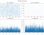
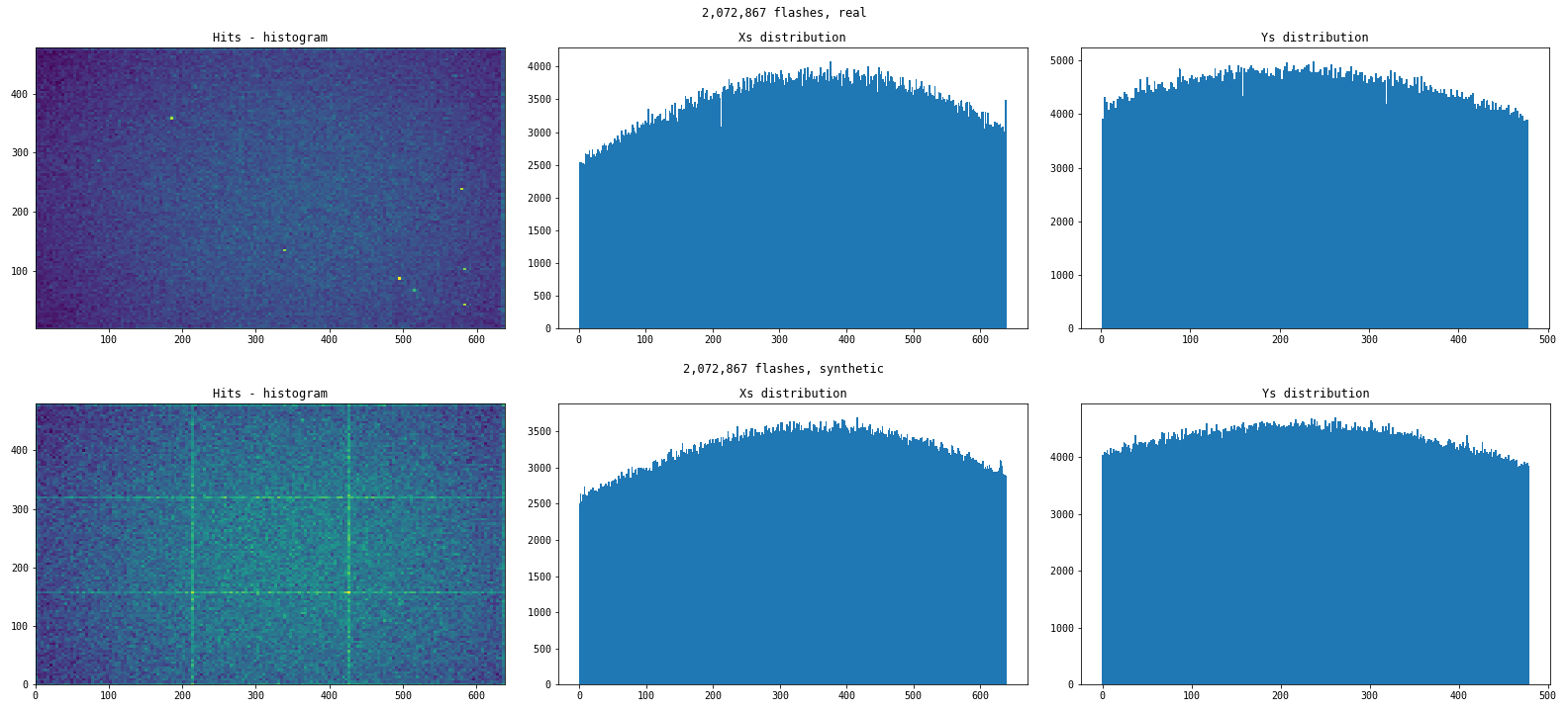
To create the following charts, I simulated big datasets of points so that it would be enough to generate 3 megabytes of output with each method. The dataset generation rules are loosely based on previously collected real data distribution patterns, including artifacts similar to hot pixels.
Here is how the actual datasets vs synthetic ones look in comparison:
-
- Good distribution
-
- Dot artifact
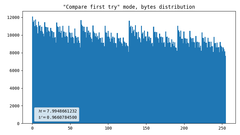
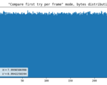
First attempt, comparator
As I needed to make things work first, I had an idea off the top of my head. It might have been inspired by an article I read a long time ago. It was something about comparing the characteristics of two photons, but I can’t find the link anymore. It is most likely that I misinterpreted the article, hence the method came out to be quite ineffective. It simply compares percentiles of X and Y coordinates of a registered flash. The yield is 2 bits per flash.
-
- Almost perfect data
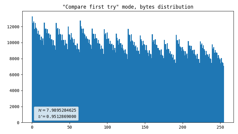
-
- Dot artifact
-
- Line artifact

Comparator, inter-frame
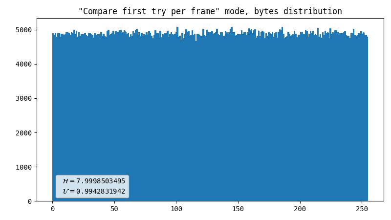
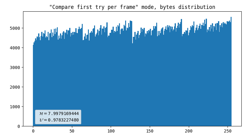
This compares the percentile of YUV coordinates within one frame with the same metric of a previous frame. Surprisingly, this produces way better results than the previous method, in terms of uniformity, not speed. The output is 1 bit for every 2 flashes.
-

- Almost perfect data
-
- Dot artifact
-
- Line artifact

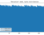
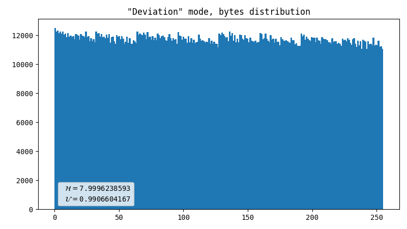
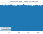
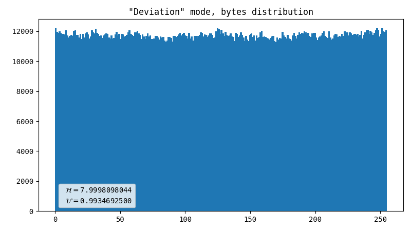
Deviation direction
This is a known method for handling Geiger counter output: we measure some value and produce either 1 or 0, which depends on the direction of deviation of that value from the mean. As we have two normally distributed values (X and Y coordinates), we can produce two bits per flash. Because the mean value is not centered, we reject flashes farther away than the nearest screen edge.
-
- Almost perfect data
-
- Dot artifact
-
- Line artifact

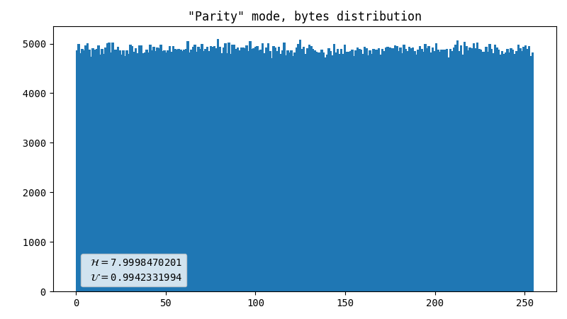
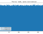
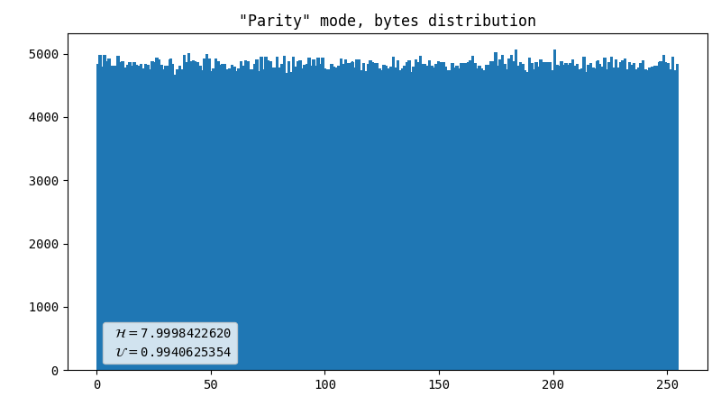
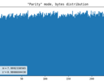
Parity (default)
I borrowed this method here. We get parity bits of X and Y coordinates, apply a simple de-skew logic, and compare the resulting values. If the least significant bits are equal, we discard both values. We output 0 when X is even and 1 when it’s odd (or the other way around, it’s not important) otherwise.
-
- Almost perfect data
-
- Dot artifact
-
- Line artifact

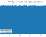
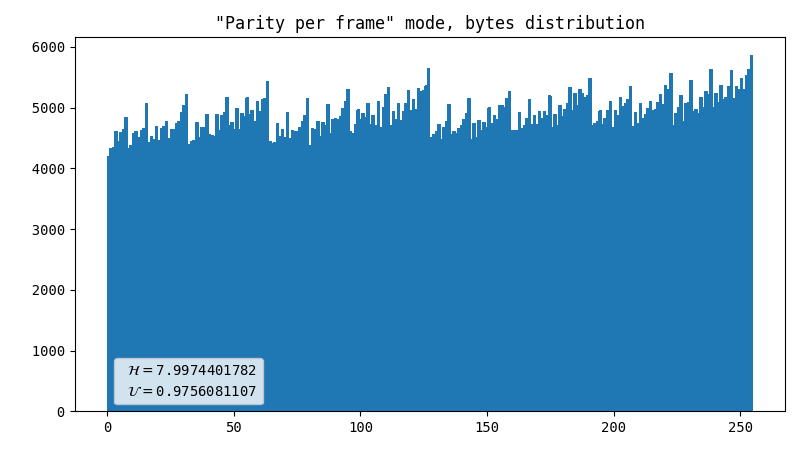
Parity, inter-frame
This is just like the simple parity check, but it compares the variables in pairs: X1 to X2 and Y1 to Y2 for consequent frames. Frankly, I was shocked by the fact that it shows such a noticeable difference compared to the previous method.
-
- Almost perfect data

-
- Dot artifact
-
- Line artifact
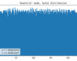
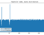
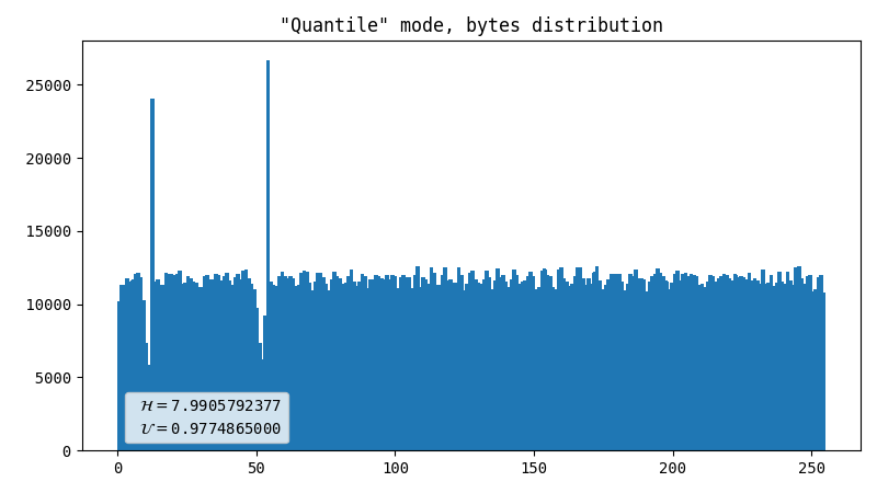
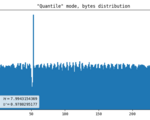
Inverse probability integral transform
If R is a random variable with CDF=F(R), then F-1(R) is a uniform(0, 1) distribution. We can form the empirical distribution function with enough independent observations of R (Knuth, 1997). So we figure out two quantile functions for X and Y respectively, based on observations of a few flashes and derive byte values from them. This produces 2 bytes per flash.
-
- Almost perfect data

-
- Dot artifact
-
- Line artifact
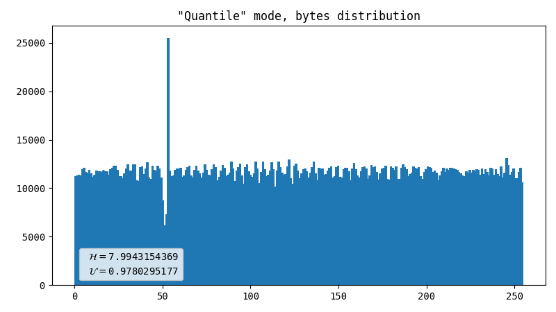
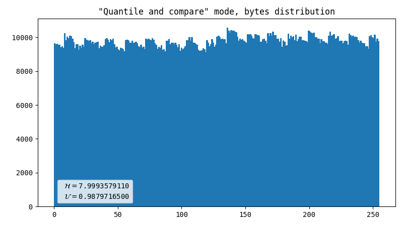
Quantile with a comparator
Previous method output looks like something relatively uniform, but with uneven gaps inside. Also, it does not resemble the normal distribution it used to be. So this method uses inverse probability integral transformation to smooth out values, and compares two uniformly distributed probabilities to generate a bit. Apparently it helps, but still it’s far from perfect.
-
- Almost perfect data

-
- Dot artifact

-
- Line artifact
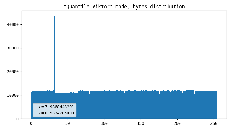
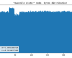
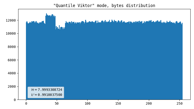
Viktor’s advice
I asked my friend for help, and among many other things he suggested another approach. The idea behind it is that we have enough entropy in raw image to be able to produce quite a lot of output, and it’s possible to find a balance between uniformity and throughput. We figured out that gluing two bytes together works pretty well. Unfortunately, this method is prone to errors when raw data has imperfections such as hot pixels.
-
- Almost perfect data

-
- Dot artifact
-
- Line artifact
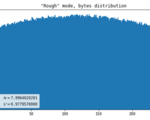
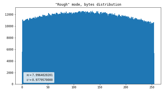
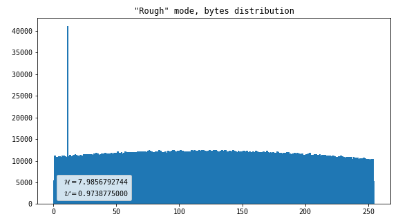
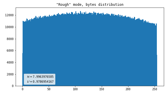
Rough
This merely converts input coordinates to output bytes without attempting to do any normalization whatsoever. The output is one byte per flash.
-
- Almost perfect data
-
- Dot artifact
-
- Line artifact
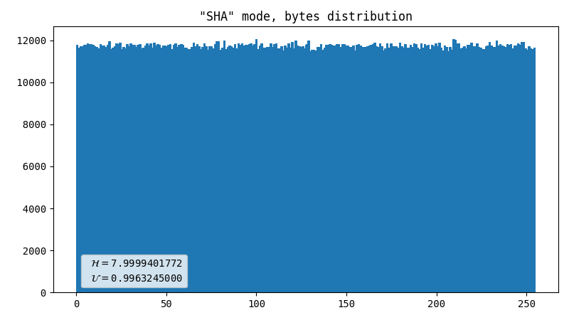
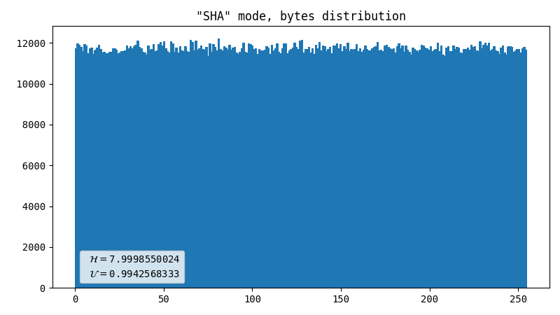
SHA-256
This automatically solves the problem with uniformity as SHA-256 (as well as any other crypto hash) produces output that is practically indistinguishable from uniform random noise. Given that each frame has WIDTH*HEIGHT*2 bytes, which is way more than the hash digest length, it should work brilliantly. If we only accept frames with at least one registered flash, it is guaranteed that at least one byte is truly random.
-
- Almost perfect data
-
- Dot artifact
-
- Line artifact

Connected components
After days of experiments, it occurred to me that eventually it will be necessary to measure the exact effect of primitive multi-pixel flash coordinates, rounding on resulting values. So I wrote this little cca.py script. The main app wasn’t fitted for writing logs exactly as Ineeded them, and it wasn’t possible to restore point relationships to the corresponding frames, so I took a few shortcuts hoping it would not mess up the results too much. What I discovered was this picture:
##    221023 (46.0498%)         #      6331 (1.3191%)            #    1887 (0.3932%)
##                              ##                              #

#      48072 (10.0157%)          ##    6226 (1.2972%)           #     1851 (0.3857%)
                                ###                              #

##     39673 (8.2658%)
                                ###    6163 (1.2841%)           ###   1152 (0.24%)
                                 ##                              #
#      34683 (7.2262%)
#
                                ##     6144 (1.2801%)            #    1113 (0.2319%)
                                ###                             ###
###    15135 (3.1534%)
###
                                                                ##    1112 (0.2317%)
                                                                ##
####    6923 (1.4424%)          ###    6104 (1.2718%)            #
####                            ##

                                                                ##    1102 (0.2296%)
##      6637 (1.3828%)          ##     5546 (1.1555%)           ##
 #                              ###                             #
                                 ##

 #      6601 (1.3753%)                                          ###   1102 (0.2296%)
##                               ##    5492 (1.1443%)           #
                                ###
                                ##
##      6470 (1.348%)                                            #    1085 (0.2261%)
#                                                               ##
                                ###    4672 (0.9734%)           ##
I had hoped the numbers would be different, but apparently the percentage of patterns affected by coordinate rounding is huge. Not only the square pattern above would be translated to the coordinates of its leftmost top pixel, but nearly 79% of all registered flashes would lead to resulting numbers being biased towards 0:0.
Once I implemented the connected components algorithm, the situation changed appreciably for the better. Now all detected flashes come down to a single coordinate, no matter how big the spot is. I tried to avoid bias in round-robin fashion so that each pixel of that square pattern above, for example, would have an equal chance to be selected. As long as the exact time of appearance and shape of such patterns remains unpredictable, I wouldn’t consider this way of data handling to be a significant threat to the quality of produced data
Benchmarks
I processed two different groups of datasets with all methods I had available at the time. One group is created synthetically so that the output would be larger than 3 megabytes. The other one is actual data collected in multiple runs, during longer periods of time.
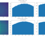
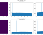
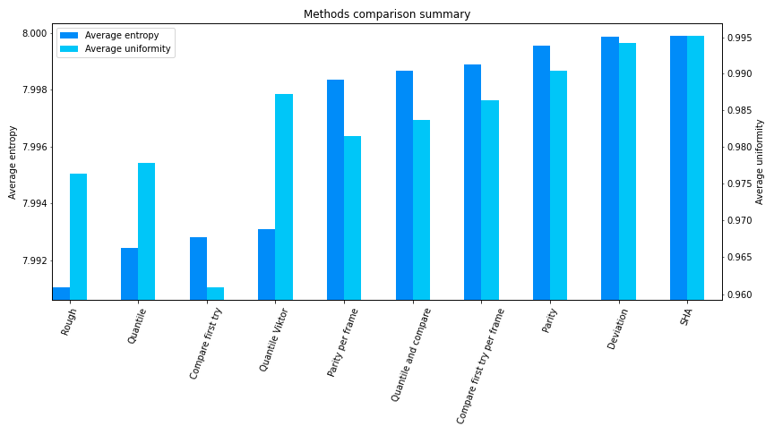
Entropy and uniformity
There is a difference between real and synthetic data, and there are two reasons for this. First of all, synthetic datasets were intentionally designed to have exaggerated defects. Secondly, the amount of collected data differs in real datasets, and the gap is enormous between real and synthetic ones. Hence, entropy and uniformity indices might be not fully converged, especially for real datasets.
-
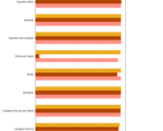
- Entropy, real data

-
- Entropy, synthetic tests

-
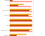
- Uniformity, real data
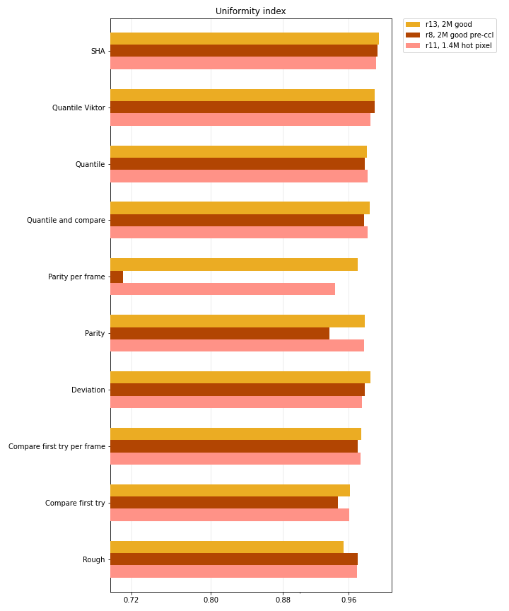
-
- Uniformity, synthetic tests

Speed
- Running time: 1 hour
- FPS: 29.5
- Average flashes per hour: 7627, per minute: 127
Interestingly enough, 127 flashes per minute is pretty consistent with what we measured at first, which was some number of flashes every 16 frames. The difference is only about 10%, and it is caused by the CCL algorithm.
| Method | Bytes per flash ratio | Bytes generated | Bytes per minute |
|---|---|---|---|
| Parity | 1/8 (with many rejects) | 800 | 14 |
| Compare first try | 1/8 | 1624 | 27 |
| Deviation | 1/8 (less rejects) | 2766 | 46 |
| Rough | 1 | 6829 | 114 |
| SHA-256 | 32 | 200192 | 3337 |
| SHA-256, all frames | approx. 512 | 3390336 | 56506 |
That’s about it for now. Have fun! :)
Credits
- Viktor Klyestov
- I also want to thank Chris Flanders, who reviewed the article and suggested corrections for it.
References
Source code:
Similar projects:
- http://etoan.com/random-number-generation/index.html
- http://www.inventgeek.com/alpha-radiation-visualizer/
- https://github.com/bitplane/schrodingers-rng
Other:
- Knuth, D. (1997). Art of Computer Programming, Volume 2: Seminumerical Algorithms (3rd ed.). Addison-Wesley Professional.
- https://www.fourmilab.ch/random/
- https://webhome.phy.duke.edu/~rgb/General/dieharder.php
- https://andor.oxinst.com/learning/view/article/ccd-blemishes-and-non-uniformities
- https://www.eso.org/~ohainaut/ccd/CCD_artifacts.html
- https://stats.stackexchange.com/a/67138
- https://stats.stackexchange.com/a/176957
- https://crypto.stackexchange.com/questions/5542/webcam-random-number-generator/